
Context Windows and Attention Budgets: Signal, Noise, Relevance, and Token Tradeoffs
The request fits. It returns a worse answer than the shorter prompt you shipped last week.

Key topics
The request fits. It returns a worse answer than the shorter prompt you shipped last week.
That is the symptom that breaks the storage metaphor. If a context window were memory, a request that fits would be a request that works. It isn't. The window is capacity, and capacity is only half the story. The other half is what each token costs you in attention, latency, and money — and how much of that cost buys signal versus noise.
I want one diagnostic handle for the rest of this article: the attention budget. Treat it as an application-level allocation heuristic, not a scalar the model reports. Every token you place in the window competes for the model's finite attention and consumes real inference resources. The engineering question is never "does it fit?" It is "does this token earn its place?"
Before we go further, one boundary matters. "Attention budget" is a design metaphor, and it sits on top of several distinct mechanisms that are easy to collapse into one:
- Context-window capacity — the hard token ceiling for a single forward pass.
- Inference compute — prefill and decode cost, which scale differently with length.
- KV-cache memory traffic — the bandwidth cost of moving cached key/value tensors during generation.
- Provider billing and runtime — pricing, caching discounts, and overflow behavior.
- Model attention weights — what the network actually attends to internally.
The metaphor helps you allocate. It does not predict any single one of those numbers. Keep the layers separate and the rest of this article stays honest.
The Window Is Capacity, Not Memory
A context window is the maximum number of tokens a model can attend to in a single forward pass — including the response it is about to generate. It is not a persistent store. It is a working set rebuilt on every call.
That single fact has a consequence most engineers learn the hard way: output competes with input for the same budget. A request that "barely fits" on input fails the moment the model emits its first output token. If you fill 120K of a 128K window with retrieved chunks and history, you have not built a rich prompt. You have built a prompt with an 8K answer budget, and long analyses, code generation, and structured responses will not fit.
The window is shared across every component you send:
- system prompt and instructions
- tool schemas and function definitions
- conversation history
- retrieved chunks and documents
- the current user turn
- reserved output tokens
Each draws from the same pool. When one grows, another shrinks. There is no separate "memory" region you can expand independently.
Two distinctions matter here, and conflating them causes most budgeting mistakes:
| Concept | Question it answers | What it determines |
|---|---|---|
| Capacity | How much fits? | Whether the request succeeds at all |
| Consumption | What does each token cost? | Latency, price, and quality degradation |
Capacity is a ceiling. Consumption is a curve. A larger window raises the ceiling; it does not flatten the curve.
One caveat before we go further: window sizes, long-context pricing, and per-model behavior differ by provider and version. Treat any specific number you read — including the ones in this article — as configuration, not a constant. The mechanism is stable. The numbers are not.
Knowledge check
Check your understanding
Answer this question before you continue.
Why Attention Has a Price Curve
The ceiling exists because of how attention works. In standard self-attention, every token compares against every other token. Compute and memory grow roughly quadratically with sequence length. Double the input, and you are closer to a 4x cost than a 2x cost.
That is the raw mechanism. Modern long-context models attack it from several directions:
- Sparse and sliding-window attention — each token attends to a subset rather than everything.
- Grouped-query attention (GQA) — multiple query heads share key/value projections, shrinking the KV cache.
- FlashAttention-style kernels — same math, better memory movement, less overhead.
- KV caching — reuse the key/value tensors computed during prefill instead of recomputing them.
These reduce the constant and the growth rate. They do not remove the ceiling. Three practical limits remain: the quadratic term still dominates at extreme lengths, quality degrades past the training distribution, and serving cost scales with the tokens you actually send.
The cost story splits into two phases, and conflating them is a common source of bad intuition.
Prefill processes the whole prompt in parallel. This is where the quadratic attention term bites hardest, and where a long prompt costs the most raw compute. Decode generates one token at a time, and here the dominant cost is often memory-bound, not compute-bound. The KV cache grows with sequence length and must be moved through memory on every step. That is why long-context latency is not just a compute story — it is a bandwidth story.
This split also explains cached-prefix discounts. When the prefill K/V for a shared prefix is already in memory, reuse is genuinely cheaper than reconstruction. That is a runtime and billing consequence, not evidence about where the model's attention goes. Caching changes what you pay. It does not change the quality tradeoff of sending extra tokens.
There is a second-order effect worth internalizing. A "long-context release" is usually not the same model with a bigger number. It has often been retrained or re-tuned with different position encoding, different attention patterns, or both. Compared to its short-context sibling, it can be slower per token, more expensive to serve, and sometimes weaker on short-context tasks. Bigger window is a tradeoff, not a free upgrade.
Knowledge check
Check your understanding
Answer this question before you continue.
Context Rot: More Tokens, Less Recall
Here is the failure the storage metaphor cannot explain. As token count grows, accuracy and recall degrade — even when everything technically fits. Providers describe this as context rot, and it is not a bug in one model. It is a property of the mechanism.
Two forces drive it.
Position matters. Retrieval accuracy tends to be strongest near the beginning and end of the context and weakest in the middle. This is the well-known lost-in-the-middle effect, and it shows up across model families. If your decisive evidence is buried at token 40,000 of a 90,000-token prompt, you have placed it in the least reliable region of the window.
Interference matters more. Semantically similar but non-decisive tokens compete with the evidence the model actually needs. Ten near-duplicate chunks about authentication do not reinforce each other. They dilute the one chunk that answers the question. This is context noise, and it is the mechanism I reach for most often when a long prompt underperforms a short one.
Separate the failure sources, because each has a different fix:
| Failure source | Symptom | Fix |
|---|---|---|
| Capacity overflow | Hard error, truncation, or empty output | Reserve output tokens; shrink input |
| Positional degradation | Correct evidence present but ignored | Move high-value evidence to the edges |
| Relevance dilution | Model hedges, blends, or picks wrong evidence | Rank, filter, and cut before packing |
| Semantic conflict or staleness | Model follows the wrong instruction or an obsolete fact | Assign authority, freshness, and provenance; isolate or replace stale state |
That last row is the one token budgeting cannot fix. A prompt can fit, contain relevant evidence, and still fail because retrieved text contradicts a system instruction, history carries a superseded value, or a tool result disagrees with the user turn. No amount of trimming or reordering resolves a conflict — you have to decide which source wins and encode that decision in the context itself.
If you treat all four as "the prompt is too long," you will apply the wrong fix. Cutting tokens helps capacity overflow. Reordering helps positional degradation. Only selection and filtering help relevance dilution — and cutting the wrong tokens makes dilution worse. Only authority and freshness rules help conflict.
The reliable working range of a model is not its advertised window size. It depends on the model, the task, and how you order the context. Treat those as two different numbers and measure the second one yourself.
Knowledge check
Check your understanding
Answer this question before you continue.
Budgeting a Request: A Worked Allocation
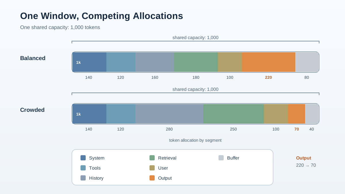
Let's make this concrete. Take a single request against a 128K-token window and allocate it component by component.
| Component | Tokens | Notes |
|---|---|---|
| System prompt | 2,000 | Instructions, persona, format rules |
| Tool schemas | 4,000 | JSON definitions for available tools |
| Conversation history | 20,000 | Prior turns, including tool results |
| Retrieved chunks | 40,000 | Top-k documents after ranking |
| User turn | 1,500 | Current question |
| Reserved output | 32,000 | Room for the model to actually answer |
| Safety buffer | 4,000 | Absorbs estimation error |
| Total | 103,500 | Leaves ~24,500 headroom |
Now run the same request against a 200K window. The shape does not change. The system prompt is still 2,000 tokens. The retrieved chunks are still 40,000. What changes is the ceiling — you now have more headroom, which means you could retrieve more chunks. That is exactly the trap. A larger window does not change the tradeoff; it changes how much rope you have.
The most common budgeting mistake is under-reserving output. If you fill 120K of a 128K window with input, the model has 8K tokens to answer — and long analyses, multi-file code generation, and structured responses routinely need 16K–64K. The request does not fail loudly. It fails by truncating the answer mid-sentence, or by producing a shallow response because the model is compressing to fit.
You cannot budget what you do not measure. Instrument token counts per component and log them per call:
def log_context_budget(
    components: dict[str, int],
    window: int,
    min_output_tokens: int,
):
    input_tokens = sum(components.values())
    usable = window - min_output_tokens
    utilization = input_tokens / usable if usable > 0 else float("inf")
    print(
        f"input={input_tokens} usable={usable} "
        f"input_capacity_utilization={utilization:.2%}"
    )
    for name, count in sorted(components.items(), key=lambda kv: -kv[1]):
        print(f"  {name}: {count} ({count / input_tokens:.1%} of input)")
    if utilization > 0.9:
        print("  WARNING: input is crowding the output budget")
Two things to notice. First, the metric is named input_capacity_utilization, not "utilization," because it measures headroom pressure — not answer quality. A 90% input utilization may be safe for a short classification and unsafe for a long structured response. Second, min_output_tokens is a required argument, not a default. The output budget is a task property, not a constant. Set it from the shape of the answer you actually need.
Run this on a real session and watch which component grows silently. It is almost never the system prompt. It is history and tool output, accumulating one turn at a time.
Two details that catch people:
- Multimodal tokens count against the same budget. Images are not free. They consume window space like any other token.
- Thinking or reasoning blocks may or may not persist across turns. On some models, previous reasoning blocks are retained and count toward the window; on others, they are stripped. Check the behavior for your specific model, because it changes your effective budget by a large margin.
Relevance Beats Volume in Retrieval Payloads
Retrieval is context selection. Every irrelevant chunk spends attention budget that the decisive evidence needed. That sentence is the whole section, but the decision rule behind it is worth spelling out.
Before comparing retrieval strategies, define the decision axis: does this task need broad coverage, or precise recall of a few facts? The answer determines everything downstream.
- For a task with a small, known answer set — "what is the refund window for this order?" — a tight curated payload of two or three high-precision chunks outperforms a large recall-oriented one. Breadth adds noise, and noise dilutes.
- For a genuinely global synthesis task — "summarize the themes across these forty documents" — breadth may be worth the dilution cost. You need coverage, and the model is doing aggregation rather than pinpoint retrieval.
Ranking and filtering before packing usually beats packing more and hoping the model sorts it out. The model is not a relevance filter you can delegate to. It is a consumer of whatever you hand it.
Ordering is a second lever. Place the highest-value evidence at the edges of the context — the beginning or the end — rather than burying it mid-prompt. This is a direct response to the positional degradation we covered earlier. If you know the middle is the weakest region, stop putting your best evidence there.
The default failure mode of retrieval is not "too few chunks." It is "enough chunks to dilute the one that mattered."
Knowledge check
Check your understanding
Answer this question before you continue.
Managing the Budget Over Long Horizons
Single-request budgeting is the easy case. Multi-turn and agentic sessions are where the budget quietly fills with stale tokens.
Long sessions accumulate history, tool output, and intermediate state. Without management, the window fills with tokens that were relevant three turns ago and are now dead weight. Two strategies dominate, and they are not interchangeable:
Compaction summarizes earlier conversation to reclaim space. It is lossy, and the loss is usually invisible until a later turn needs a discarded detail. Compaction buys capacity at the cost of fidelity. Use it when the conversation genuinely needs to continue past the window, and accept that some information will not survive.
Isolation keeps bulky artifacts outside the prompt and passes handles instead. The window holds a reference — a file path, a document ID, a tool result key — rather than the payload itself. This is the alternative to compression, and for many agent workloads it is the better one. You are not summarizing the artifact; you are declining to load it until it is needed.
Some models expose context-awareness features that report remaining budget, injecting token-usage warnings into the conversation. These are convenient, but they are not a substitute for your own accounting. Availability varies by model, and you should not build your budget logic on a feature that may not exist on the model you switch to next quarter.
The failure path to plan for is overflow behavior, which differs by platform:
- Hard error — the request fails loudly. Annoying, but honest.
- Silent truncation — tokens are dropped without warning. The worst case, because it hides the bug.
- Client-side summarization — the harness compacts before sending. Convenient, but it can discard exactly the detail you needed.
Each hides a different class of bug. Know which one your stack does.
Measuring Your Own Attention Budget
The budget model is only useful if it is observable. Build a probe — but build the right one, because a single retrieval curve does not establish that your production task will improve.
Start with a needle-in-a-haystack test. It places a known fact at varying positions and context lengths, then measures retrieval accuracy as a curve rather than a single number:
- Choose a target fact — a unique string or number.
- Embed it at a controlled position (10%, 50%, 90%) within a context of controlled length.
- Fill the rest with realistic distractor chunks, not random text.
- Ask the model to retrieve the fact.
- Record accuracy, latency, and cost per configuration.
Vary one axis at a time — position, total length, number of distractors — so you can attribute degradation to the right cause. If accuracy drops when you add distractors but holds when you extend length, you have a relevance problem, not a capacity problem. That distinction changes your fix.
Then be honest about what the needle test cannot tell you. It measures known-fact retrieval. It does not measure instruction conflict, multi-hop evidence, aggregation, tool-call correctness, answer completeness, or recovery after compaction. A production system can pass the needle test and still fail on any of those.
So extend the probe into a task-level ladder. Each rung tests a different capability, and each has its own success signal:
| Capability | Probe | What it establishes |
|---|---|---|
| Retrieval | Needle at varied positions | Whether the fact survives the context |
| Synthesis | Multi-hop question over several chunks | Whether the model combines evidence |
| Instruction-following | Conflicting instruction vs. retrieved text | Whether authority rules hold |
| Tool use | Task requiring a correct tool call | Whether schemas and results survive |
| Recovery | Task after a compaction event | Whether discarded detail mattered |
Run the ladder before you change a context policy. If retrieval holds but synthesis fails, the problem is not capacity — it is how evidence is selected and ordered. If instruction-following fails, the problem is authority, not length.
Track cost and latency alongside accuracy. A configuration that improves recall by a few points at three times the input cost is usually the wrong trade. The point of the probe is not to find the maximum-accuracy configuration. It is to find the configuration where marginal accuracy stops justifying marginal cost.
Log per-component token counts and per-call cost so regressions surface as data rather than as vague quality complaints. When someone says "the answers got worse last week," you want a token-count chart, not a debate.
Treat benchmark and vendor claims as conditions, not guarantees. Your task, your ordering, and your distractor distribution determine your real working range. A model that scores well on a published long-context benchmark may behave differently on your retrieval payload, because your payload has different noise characteristics.
The Decision Rule
Treat the window as a budget you allocate per decision, not a tank you fill. Every token is a bid for attention, and the model pays for all of them whether they help or not.
The next action is concrete. On your next request, instrument token counts for each context component — system, tools, history, retrieved chunks, user turn, reserved output — and log them per call. Watch which component grows across a session. Then run a position-varied retrieval probe to find your model's real working range, not its advertised one. When the probe passes but the task still fails, move up the ladder: synthesis, instruction-following, tool use, recovery.
One boundary condition: when the task genuinely needs global synthesis across a large corpus, breadth can be worth the dilution cost. That is a legitimate choice. But it should be a measured choice, backed by a probe that shows the breadth is buying accuracy you cannot get from a tighter payload — not a default you fall into because the window was big enough to allow it.
Knowledge check
Final check
Finish the article by checking the ideas you just learned.
References
Research updated Sep 11, 2026


