Search and Tree Loops: Branching, Backtracking, Beam Search, MCTS, and LATS

A linear agent loop is a commitment device. It commits to one trajectory, and every later step inherits the consequences of the earliest mistake.

Watch a ReAct-style agent fail on a multi-step task and you will usually see the same shape. The first tool call is plausible but wrong. The observation that comes back is ambiguous enough to pass. The second call builds on the first, the third builds on the second, and by the time the evidence is unmistakable, the trajectory is already poisoned. The agent is not stuck because it reasoned poorly at step seven. It is stuck because step one is load-bearing and nothing in the loop can put it down.

The weak mental model behind this failure is that the agent's job is to pick the next best action. That model produces a single-threaded loop, and a single-threaded loop has no recovery surface. The stronger model is that the agent's job is to maintain a frontier of candidate states and decide where to spend the next unit of compute. Once you accept that framing, "what is the next action" becomes a special case of "which node do I expand," and the whole family of tree search agent loops becomes available.

This article compares that family along four axes: state evaluation (what scores a node), budget (what bounds the search), rollout quality (how a leaf value is estimated), and recovery behavior (what happens after a dead end). Every strategy below is a different answer to those four questions.

Why a Linear Loop Cannot Recover

Backtracking is not a feature you bolt onto a loop. It requires three things a linear loop does not have.

First, a stored frontier. If you only keep the current state, there is nowhere to go back to. Second, a way to score a partial state. If you cannot rank an unfinished trajectory against another unfinished trajectory, "go back" is just "try something else." Third, a policy for choosing which node to expand next. Without it, you have a bag of candidates and no reason to prefer any of them.

A wrong early action is not a wrong step. It is a corrupted state that every later step inherits. Backtracking is the only mechanism that lets the loop discard the state without discarding the work that produced it.

The decision boundary is economic. Tree search pays off when the cost of a wrong early commitment exceeds the cost of exploring alternatives. If your task is a single tool call, or if the environment cannot be reset or replayed, or if your evaluator is no better than a coin flip, tree search is not a smarter loop. It is a more expensive way to be wrong.

The Shared Skeleton: Search Control, Not Just Evaluation

Every strategy in this article is a variation on one loop, but the loop is not "evaluate and pick." Search control decomposes into six components, and each named strategy changes a different subset.

frontier = [root_state]
while budget_remaining():
    node = select(frontier)              # selection policy
    children = propose(node)             # proposal policy: candidate actions
    for child in children:
        child.state = transition(node, child.action)  # environment step
        child.value = evaluate(child)    # evaluator: partial-state score
    backup(node, children)               # value propagation
    if terminal(best_child):
        return best_child

The node is a state. The edge is an action. But the model's judgment enters at four distinct points: propose (which actions to try), transition (how the environment responds), evaluate (how good a partial state looks), and backup (how leaf values aggregate). Calling the value function "the only place the model's judgment enters" is wrong for LATS, where the model also generates reflections that change future proposals, and wrong for any agent where observation interpretation shapes the next expansion.

Keep the search tree separate from the agent's memory. The tree is ephemeral working state: nodes, edges, visit counts, backed-up values. The durable context the model sees is a different object, assembled from the current node's path plus whatever reflection or summary you choose to carry forward. Conflating them is the most common implementation mistake, because it makes the tree grow into the prompt until the context window is the real budget.

The State/Replay Invariant

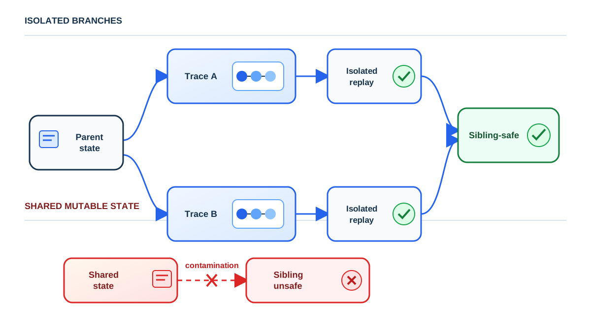
Backtracking is only real if a branch can be resumed without contaminating its siblings. That requires a node record that is either a replayable snapshot or a reconstructable trace. The minimum node record:

node = {
  state_snapshot:  environment state at this node (or None if not snapshotable)
  action_trace:    ordered list of actions from root to this node
  observations:    tool results and environment feedback along the trace
  value:           evaluator score
  visits:          expansion count (for UCT-style selection)
  parent:          pointer for backup
}

For pure or replayable tasks — code execution in a sandbox, math, read-only retrieval — you can reconstruct any node by replaying its action trace from the root. For side-effecting environments — file writes, API calls that mutate state, purchases — replaying a trace duplicates the side effect. Two nominally identical nodes then behave differently, and your search is silently corrupt.

If your tools mutate external state, search over plans or tool-call proposals first. Validate the selected path once, then execute it. Do not branch over destructive actions unless you have snapshots, compensating actions, or a sandbox that absorbs the side effects.

This builds on the state/action/observation/termination contract from the anatomy of an agent loop. Assume that contract. What changes here is that select, backup, and the replay invariant now have real work to do.

Greedy and Beam: Branching Without Memory

Greedy best-first is the cheapest search you can build. Generate a set of candidate actions, execute them, score the results, keep the single best, repeat. It branches, but it does not remember. Abandoned branches are gone.

Beam search keeps the top-k frontier at each depth. It is level-synchronized: expand every node in the current beam, score all children, keep the top k, discard the rest. The beam width is the budget knob, and it is a fixed-width commitment: you spend the same k candidates on a step where the decision is obvious and on a step where the decision is genuinely uncertain. A correct branch can be pruned early because the heuristic that scores partial states is weakest exactly when the branch has the least evidence behind it.

Axis	Greedy best-first	Beam search
Frontier memory	Current node only	Top-k nodes at current depth
Expansion width	Branching factor per step	Beam width × depth
Selection rule	Argmax of child scores	Top-k of child scores
Lookahead	None	None
Backup	None	None
Recovery	None	None; pruned branches discarded

Use these when the decision space is shallow, actions are cheap, or you need a fast baseline before paying for MCTS. A beam of width 2 is often enough to catch the single catastrophic early commitment that a greedy loop would have walked into.

A* and Heuristic Search: Backtracking With a Cost Model

A* adds two terms: cost-so-far, and a heuristic estimate of remaining cost. That combination makes backtracking principled rather than random. The search can return to a previously abandoned node because the node's estimated total cost is now competitive with the frontier.

For reward-maximizing agent tasks, translate the objective: minimize cost_so_far + heuristic_remaining_cost, or equivalently maximize reward_so_far + heuristic_remaining_reward. The direction matters. If you mix a cost-minimization heuristic with a reward-maximization evaluator, the search will prefer nodes that look cheap and score high, which is not the same thing as nodes that lead to success.

The heuristic is the whole game. A weak LLM-generated heuristic turns A* into an expensive greedy search with extra bookkeeping. A defensible heuristic requires a real cost signal: steps taken, tokens spent, distance to a measurable goal. If you cannot defend the heuristic, you are paying for the bookkeeping without buying the guidance.

Recovery behavior is the key limitation. A* can revisit an abandoned node, but it does not update its strategy from the trajectories it has already run. It does not learn that a particular kind of action keeps failing. Worst-case LLM calls exceed greedy, but the search is still bounded by the frontier size and by the heuristic's admissibility assumptions.

Use A* when the task has a real cost signal and a heuristic you can defend. It is the middle ground between a fast dumb search and a slow smart one.

MCTS: Spending Budget Where Uncertainty Lives

Monte Carlo Tree Search changes the selection rule. Instead of expanding the best-scoring node, it expands the node that maximizes an upper-confidence bound: exploitation of high-value nodes plus an exploration bonus for under-visited ones. The exploration constant is the real tuning surface, and it controls how much the search is willing to spend on nodes that look mediocre but have not been tried enough to know.

Rollouts estimate a leaf's value. Rollout quality is the dominant source of error when the policy used for simulation is weak, because a bad rollout produces a bad value, and a bad value corrupts the backup.

Backpropagation aggregates values up the path. A single good leaf can raise the score of an entire prefix, which is what enables reuse of partial successes: the search does not throw away a promising sequence of actions just because the final step failed.

Failure mode: a noisy or biased value function makes the confidence bound chase noise. The search converges confidently on the wrong branch, and the confidence is the problem, not the symptom.

MCTS is anytime. You can stop at any node count and take the best root action. That is a genuine operational advantage over fixed-depth beam search, because it lets you trade latency for quality at runtime instead of committing to a depth in advance.

LATS: MCTS With Language Value Functions and Reflection

Language Agent Tree Search adapts MCTS to language agents by using the model as agent, state evaluator, and feedback generator, and by using environment interaction instead of a learned world model. That last choice matters: standard MCTS and its relatives often rely on an internal dynamics model to simulate, and LATS does not require one.

The reflection step is the real addition. After a failed trajectory, the system generates a reflection and feeds it into later trials as additional context. This is cross-trial memory that plain MCTS does not have. It is the mechanism that lets the search change its policy between attempts rather than just re-sampling the same distribution.

Published results are task- and model-dependent. LATS reports state-of-the-art pass@1 accuracy on programming benchmarks with GPT-4 and competitive web navigation scores with GPT-3.5, and the reported experiments show it expanding fewer nodes on success than comparable tree baselines. Treat those numbers as evidence that the approach works under specific conditions, not as a general guarantee. The per-node cost includes multiple LLM calls for evaluation and reflection, so fewer nodes does not automatically mean fewer tokens.

The failure mode is reflection that restates the failure without changing the search policy. If the reflection says "the tool call failed" and the next trial makes the same tool call, you have added tokens to the same dead branch. Reflection has to change something the search can act on: the candidate actions, the value function, or the pruning rule.

Choosing a Strategy: The Decision Table

Four axes decide the choice: the cost of a wrong early action, the quality of your state evaluator, the availability of a real cost or reward signal, and how much budget you can spend per task.

Strategy	Right default when	Overkill when
Greedy	Actions are cheap and the task is short	Any early mistake is expensive
Beam	You need a fast baseline and shallow branching	The correct branch looks weak early
A*	You have a real cost signal and a defensible heuristic	You cannot defend the heuristic
MCTS	Uncertainty is unevenly distributed across the tree	The value function is noisy or biased
LATS	Failures are informative and reflection can change policy	Reflection just restates the failure

Do not use tree search at all when the task is single-step, when the environment is not resettable or replayable, or when the evaluator is no better than chance. In that last case, more search makes the failure more expensive, not less likely.

The evaluator is the bottleneck in every strategy here. If you cannot score a partial state better than chance, branching multiplies your cost without improving your odds.

Budget, Termination, and the Cost of Recovery

Pick more than one termination condition, because any single bound can be gamed by the search. Node budget, token budget, wall-clock budget, value threshold, and depth limit each fail differently. A node budget with no value threshold will happily exhaust itself on a hopeless branch. A value threshold with no node budget will run forever if the evaluator is miscalibrated.

Log the frontier, the value distribution, and the pruning decisions. A search that never prunes is a search that is not evaluating. If every node survives to the end, your value function is not discriminating.

Detect the failure early: if the best root value stops improving across expansions, the evaluator or the branching factor is wrong, not the budget. Adding nodes to a search that has stopped improving just adds cost.

Cost accounting matters more here than in a linear loop. Tree loops multiply LLM calls by branching factor and depth, so measure cost per solved task, not cost per call. A search that uses three times the calls but solves twice as many tasks is cheaper per solve, and that is the number that shows up in production.

What to Build First

Build the evaluator before you build the tree. Take an existing linear agent task, collect a set of partial trajectories, and check whether your evaluator ranks them better than chance. But "better than chance" is a weak bar. A heuristic can rank above chance while still preferring verbose, plausible, or prematurely complete states. Verify the evaluator against outcomes: on held-out branches, compare partial-state scores with eventual task success. Inspect ranking quality at equal depth, and test whether scores favor artifacts such as length or confident language. If the evaluator is biased toward surface features, branching will amplify the bias.

Then run one concrete experiment: add a beam of width 2 with a scored frontier to a sandboxed, read-only, or simulated task you already have. Keep everything else the same. Measure solve rate, LLM calls per task, evaluator agreement with eventual success, terminal failures, and latency. If the extra calls buy a higher solve rate, you have evidence that branching is the right axis. If they do not, the problem is the evaluator, and reaching for MCTS or LATS will only make the wrong answer more expensive to find.

Start with the evaluator. Prove it ranks partial states in the right order. Then add one branch.

References

Research updated Sep 11, 2026