
Decomposition and Planning Prompts: Least-to-Most, Plan-and-Solve, and Self-Discover
The first sub-answer is wrong, and every later step inherits it with full confidence.

Key topics
The first sub-answer is wrong, and every later step inherits it with full confidence.
That is the failure that sends engineers looking for decomposition and planning prompts. A multi-step task gets one prompt, the model produces a fluent chain of reasoning, and somewhere in the middle a premise is quietly false. Nothing downstream flags it. The model does not hesitate, does not hedge, does not circle back. It builds a cathedral on a cracked foundation and hands you the keys.
The weak model behind most failed attempts is this: decomposition is just asking the model to break the task into steps. That model is incomplete. It treats decomposition as a formatting choice when it is actually a graph decision. You are choosing nodes — sub-tasks — and edges — dependencies between them. Every place you cut that graph is a place where an error either gets contained or gets amplified. The strategy is determined by the dependency structure of the task, not by which paper name sounds most advanced.
This article compares three prompt-only strategies — least-to-most, plan-and-solve, and self-discover — along three axes: dependency structure, error propagation, and execution overhead. I am assuming you already write explicit prompt contracts with inputs, constraints, outputs, and acceptance criteria. Everything here sits on top of that substrate. The question is where to cut.
Why "Break It Into Steps" Is Not a Strategy
A single early error becomes a premise for every later step, and the model does not flag it. It builds on it fluently. This is the defining failure mode of naive multi-step prompting, and it is not a reasoning failure — it is a structural one. The model has no checkpoint between steps, so it has no mechanism to catch a bad premise before it propagates.
Decomposition is a graph decision. You are choosing nodes and edges, and the shape of that graph determines where errors can be caught. Three axes matter:
Dependency structure. Are sub-tasks strictly ordered, independent, or conditionally dependent on intermediate results? A strictly ordered chain has different failure properties than a set of parallel sub-goals.
Error propagation. Does a bad step stay local or contaminate downstream? If there is no checkpoint between steps, a wrong sub-answer becomes an input to the next step, and the error compounds silently.
Execution overhead. Tokens, latency, number of model calls, and how much of the plan is wasted when execution fails. A strategy that costs five calls and fails at step four has burned four calls for nothing.
One boundary worth stating up front: prompt-only refers to how the decomposition is expressed, not to the absence of a harness. You can run any of these strategies inside a single call, a multi-call loop, or an externally validated orchestration layer. The prompt pattern determines what the model produces; the runtime determines whether anything can inspect it. Keep those two layers separate, because most of the confusion in this space comes from collapsing them.
The invariant: decomposition is a choice about where you cut the dependency graph. Every cut point is a place where an error either gets contained or gets amplified.
Least-to-Most: Decompose First, Then Solve in Order
Least-to-most prompting is a two-phase structure. Phase one produces an explicit ordered list of sub-questions from general to specific. Phase two answers them in sequence, feeding each answer into the next prompt.
The core assumption is that sub-problems are strictly ordered and each one is easier than the original problem. That invariant is what makes the strategy work. The model never has to hold the whole problem in one reasoning pass, and each sub-answer becomes visible context for the next.
Here is the shape in pseudocode:
Phase 1 — Decompose:
  Input: original problem P
  Output: ordered list [Q1, Q2, ..., Qn]
          where each Qi is easier than P
          and Q1..Qi-1 are prerequisites for Qi

Phase 2 — Solve in order:
  context = ""
  for i in 1..n:
    answer_i = model(Qi, context)
    context += answer_i
  return context
The dependency structure is strictly sequential. Error propagation follows directly: an error in sub-question 2 is silently absorbed into the prompt for sub-question 3. The basic pattern has no built-in checkpoint. The model does not know that answer 2 was wrong, so it treats it as established fact.
That is a property of the prompt pattern, not a law of the universe. If you wrap the loop in a harness that reads answer_i and can reject it before appending to context, you have added a checkpoint. The prompt did not change; the control boundary did. This distinction matters because the same least-to-most prompt can be a containment system or an amplification system depending on whether anything outside the model gets to look at the intermediate answer.
Execution overhead is N+1 model calls for N sub-problems, plus the cost of the decomposition pass itself. Latency scales linearly with decomposition depth. If your task decomposes into eight sub-questions, you are paying for nine calls and the latency of a sequential chain.
Where it breaks: tasks with parallel or independent sub-goals, and tasks where the decomposition itself is the hard part. The model can produce a plausible-looking but wrong ordering. A wrong ordering is worse than no ordering, because it gives the model false confidence in a sequence that does not match the actual dependency graph.
A practical mitigation: insert an explicit verification step between sub-answers, or require the model to restate the dependency it is relying on before answering. The restatement is cheap and it makes the dependency visible in the trace. If the model cannot articulate why Q3 depends on Q2, that is a signal the ordering may be wrong.
Knowledge check
Check your understanding
Answer this question before you continue.
Plan-and-Solve: One Plan, Then Execute Against It
Plan-and-solve separates planning from execution. A planning prompt produces a full plan up front. A second prompt — or a second pass — executes each step against that fixed plan.
The structural difference from least-to-most is that the plan is a single artifact you can inspect, log, and reject before any execution tokens are spent. That is the whole point. You get a checkpoint between planning and execution that the basic least-to-most loop does not have.
But the checkpoint is not free with the label. If the plan is generated and executed in the same context window with no external read, you have paid for the structure without gaining the checkpoint. The model sees its own plan and its own execution in the same context, and it will rationalize the execution to match the plan. The checkpoint only exists if something outside the model reads the plan and decides whether to proceed. This is the same boundary that applies to least-to-most: the prompt pattern produces an artifact; the runtime decides whether that artifact has authority.
Error propagation now has two distinct sources. A bad plan is caught early and cheaply — you read it and throw it away. A bad step execution is caught late and expensively — you have already paid for the plan and every step up to the failure. Name both, because they have different costs and different mitigations.
The plan-drift problem is the one that bites in practice. Once execution starts, the model tends to follow the plan even when an early step reveals the plan was wrong. A fixed plan is a commitment device and a liability. It keeps the model on track when the plan is good, and it keeps the model on track when the plan is bad.
Execution overhead is fewer calls than least-to-most in the happy path, but a failed plan wastes the entire planning pass and any executed steps. If the plan is wrong, you have paid for planning plus partial execution and have nothing to show for it.
A practical pattern: make the plan an explicit output contract. Numbered steps, declared inputs and outputs per step, and a stated condition under which the plan should be abandoned.
Plan output contract:
  1. <step description>
     inputs:  <what this step needs>
     outputs: <what this step produces>
  2. ...
  Abandon plan if: <condition>
The abandon condition is the part most people skip. Without it, the model has no instruction for what to do when reality diverges from the plan, so it does what models do — it continues.
Knowledge check
Check your understanding
Answer this question before you continue.
Self-Discover: Let the Model Choose Its Own Reasoning Structure
Self-discover prompting shifts the decomposition decision from the prompt author to the model. The model first selects or composes a reasoning structure — a set of atomic reasoning modules and how they combine — for the task, then applies that structure to the actual problem.
The key shift is that the decomposition is not fixed by you. The model is choosing the shape of the solution path. That is useful when you cannot predict the right structure in advance, and it is a liability when you need stable, auditable behavior.
The observable output is a structure selection: a named set of reasoning modules and a stated combination. In a two-pass implementation, that selection is emitted as text, then fed back into a second prompt that applies it. In a single-pass implementation, the selection and application happen in one generation and the structure is latent in the prose. Those are different systems. The two-pass version gives you an artifact you can log and reject; the single-pass version gives you a plausible-looking answer with no inspectable intermediate.
Why this matters for heterogeneous task batches: one prompt can serve tasks with different dependency shapes. If your workload mixes strictly ordered tasks with parallel ones and conditional ones, self-discover lets the model pick a structure per task. The cost is less control over the structure you get.
Error propagation has an extra failure point. The structure-selection step is itself a failure point. A wrong structure produces a confidently wrong answer that looks well-reasoned. The model picked a structure, applied it, and produced output that is internally consistent but externally wrong. This is harder to catch than a bad step in a known sequence, because you do not have a reference structure to compare against.
Execution overhead depends on implementation. A two-pass version adds a meta-reasoning call before any task work; a single-pass version does not. Either way, output variance is higher than the other two strategies because the structure varies per task. You cannot pre-compute cost per task when the structure is chosen at runtime. Some tasks will be cheap, some expensive, and you will not know which until the model has chosen.
Honest boundary: this is the least predictable of the three. It is a good fit for exploratory or heterogeneous workloads and a poor fit for pipelines where you need stable, auditable step counts. If your system has an SLA, self-discover is a variance problem before it is a capability problem.
The contrast with the other two is clean: least-to-most and plan-and-solve impose structure from outside; self-discover asks the model to generate it from inside.
Knowledge check
Check your understanding
Answer this question before you continue.
Choosing Between Them: A Dependency-First Decision Rule
Convert the three mechanisms into a decision procedure. Start with the dependency graph, not the technique name.
Step one: map the dependency graph. Are sub-tasks strictly ordered, independent, or conditionally dependent on intermediate results? Draw it. If you cannot draw it, you do not understand the task well enough to decompose it.
Step two: ask where an error can be caught. If there is no checkpoint between steps, you are choosing a strategy with no automatic containment guarantee. The checkpoint is the thing that matters, not the strategy label.
Step three: price the overhead. Count model calls, estimate latency, and ask what fraction of work is discarded when the plan or structure is wrong.
| Dependency shape | Strategy | Why |
|---|---|---|
| Strictly ordered, predictable | Least-to-most | Sequential chain matches the graph; each step feeds the next |
| Ordered, plan worth inspecting | Plan-and-solve | Plan artifact gives you a checkpoint before execution |
| Heterogeneous or unknown structure | Self-discover | Model picks structure per task; less control, more flexibility |
| Independent sub-tasks | None of these | Run them in parallel; decomposition adds overhead for no benefit |
That last row deserves a caveat. Independent branches can run in parallel, but the final merge is still a composition node. If three parallel branches produce three answers and you concatenate them, you have not verified that they agree, that they cover the same scope, or that the merge preserves the original intent. Parallelism moves the risk from the chain to the join. Add an acceptance check on the merged output before you declare the task done.
The hybrid case is where this gets interesting. Plan-and-solve for the outer structure with least-to-most recursion inside a step that turns out to be harder than expected. This is the pattern that scales when a single strategy stalls. The outer plan gives you a checkpoint; the inner recursion gives you depth where you need it. You pay for both, so use it when the task genuinely has mixed dependency shapes.
When not to use any of them: single-step tasks, tasks where the model's zero-shot answer is already correct, and tasks where the decomposition cost exceeds the value of the answer. Decomposition is not free and it is not always an improvement. I have watched engineers add a three-call decomposition pipeline to a task the model solved correctly in one call, then wonder why latency tripled and accuracy did not move.
If there is no checkpoint between steps, you are choosing a strategy with no automatic containment guarantee. Add the checkpoint before you add the technique.
Knowledge check
Check your understanding
Answer this question before you continue.
A Worked Trace: Where the Error Actually Lands
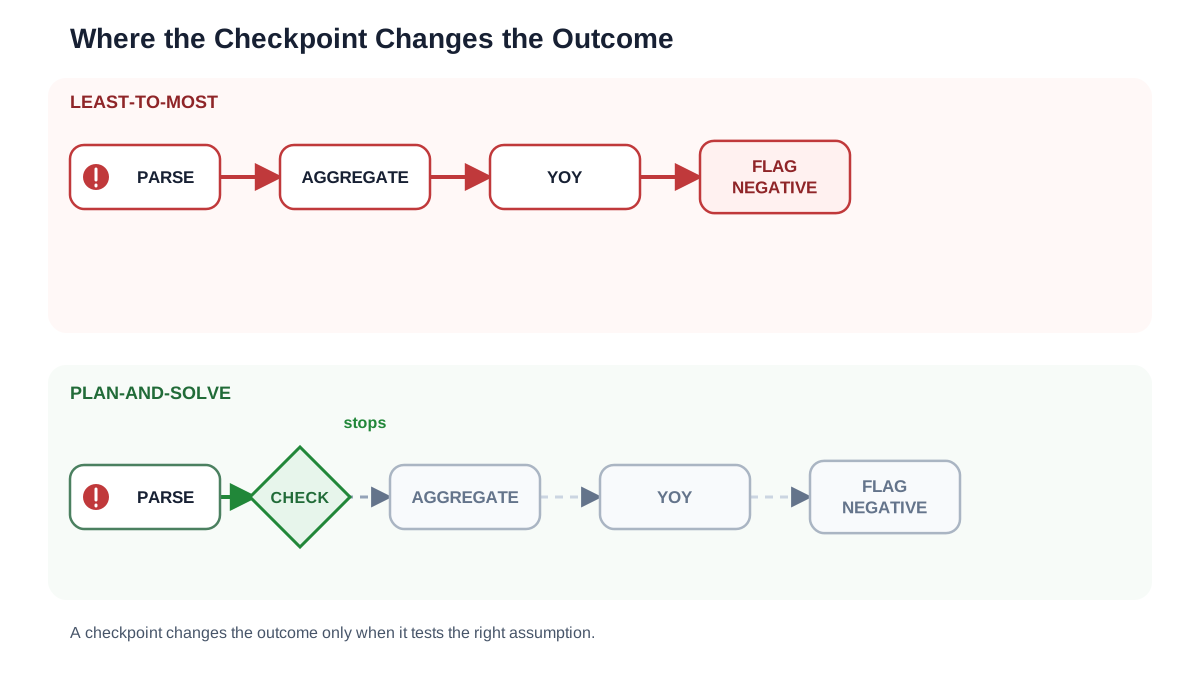
Abstract claims about propagation are easy to nod at and hard to internalize. Here is a small task with a known dependency graph, run through two strategies, with one injected fault.
Task: "Given a CSV of monthly revenue, compute the year-over-year growth rate for each quarter and flag any quarter where growth is negative."
Dependency graph: parse CSV → aggregate by quarter → compute YoY → flag negatives. Strictly ordered. Four nodes, three edges.
Least-to-most trace. Phase one produces:
Q1: What is the schema of the CSV?
Q2: How do I aggregate monthly rows into quarters?
Q3: How do I compute year-over-year growth from quarterly totals?
Q4: How do I flag negative growth quarters?
Phase two answers Q1 through Q4 in sequence. Now inject a fault: Q2's answer uses calendar quarters (Jan–Mar) when the data uses fiscal quarters starting in February. Q3 receives a quarterly aggregation that is off by one month. Q3 does not know this. It computes YoY on the wrong buckets and returns a number. Q4 flags negatives based on that number. The final answer is fluent, internally consistent, and wrong. Nothing in the chain caught the fiscal-quarter mismatch because nothing in the chain was asked to check it.
Plan-and-solve trace. The planning pass emits a plan with declared inputs and outputs per step. If the plan contract includes "confirm quarter definition from data or spec" as step 1, the fiscal-quarter mismatch is caught before aggregation runs. If the plan contract omits that step, plan-and-solve fails the same way least-to-most does — the checkpoint exists but it checked the wrong thing. This is the point: the checkpoint is only as good as the acceptance criteria you put in it.
What the trace teaches. The strategy did not determine the outcome. The presence of a checkpoint and the content of its acceptance criteria determined the outcome. Least-to-most with a harness that validates Q2's quarter definition against the spec would have caught the fault. Plan-and-solve without that check would not have. The label is not the mechanism.
Instrumenting Decomposition: What to Measure Before You Commit
Strategy choice should be evidence-based, not vibes-based. Here is the evaluation loop I would run before committing to any of the three.
Measure per-step accuracy, not just final-answer accuracy. A pipeline that is 90% correct per step is roughly 59% correct over five steps. The compounding is the whole story. If you only measure final answers, you cannot tell whether a failure came from a bad decomposition or a bad execution.
Log the decomposition artifact itself. The sub-question list, the plan, or the chosen reasoning structure. This is the only way to tell a bad decomposition from a bad execution. When a task fails, read the artifact first.
Inject a known-wrong intermediate answer and observe whether the pipeline catches it. If it never catches it, you have no error containment regardless of which strategy you picked. This is the single most informative test you can run, and it takes an afternoon.
Track cost per successful task, not cost per call. A cheap strategy that fails often is the expensive one. If least-to-most costs three calls and succeeds 70% of the time, and plan-and-solve costs four calls and succeeds 85% of the time, plan-and-solve is cheaper per success despite the higher per-call cost.
Variance matters as much as mean. Self-discover and plan-and-solve can produce good average results with wide spread. Wide spread is a problem for anything user-facing or SLA-bound. If your p95 latency is three times your p50, you have a variance problem that the average hides.
Keep the evaluation small and runnable. A dozen hand-built tasks with known correct decompositions will tell you more than a large benchmark you cannot inspect. You want to read the decomposition artifact, see where it diverged, and understand why. A benchmark score does not give you that.
The Next Move
Before choosing a strategy, draw the dependency graph and mark where an error can be caught. If there is no checkpoint, add one before you add a technique. The checkpoint is the load-bearing element; the strategy is just how you arrange the steps around it.
Take one multi-step task currently handled by a single prompt. Write down its sub-task dependency graph. Run it through least-to-most and plan-and-solve side by side, logging the decomposition artifact and per-step accuracy for both. Inject one known-wrong intermediate answer into each run and record whether the pipeline catches it. The comparison will tell you more about your task than any of the three papers can.
Then look at the failures. If the decomposition was wrong, you have a planning problem. If the decomposition was right and a step failed, you have an execution problem. If the decomposition was right and every step succeeded but the final answer was wrong, you have a composition problem — and that is the one no prompt strategy fixes.
Knowledge check
Final check
Finish the article by checking the ideas you just learned.
References
Research updated Sep 11, 2026


