
Few-Shot Example Engineering: Selection, Ordering, Diversity, and Boundary Cases
Your few-shot set passes every happy-path test, then folds the moment a real input arrives with an extra clause, an unusual label, or a phrasing you did…

Key topics
Your few-shot set passes every happy-path test, then folds the moment a real input arrives with an extra clause, an unusual label, or a phrasing you did not anticipate. The examples looked fine. The model did exactly what the examples taught it to do.
That is the uncomfortable part. A demonstration set is not a style guide. It is a small labeled training set that lives inside the context window, and the model will fit whatever pattern is cheapest to extract from it — including the ones you never meant to include. Few-shot example engineering is the discipline of controlling that signal: choosing which inputs to show, in what order, with what diversity, and which boundaries to expose so the model learns the mapping instead of a coincidence.
This assumes you already know that examples change behavior. The question here is which examples, and why.
The Control Loop
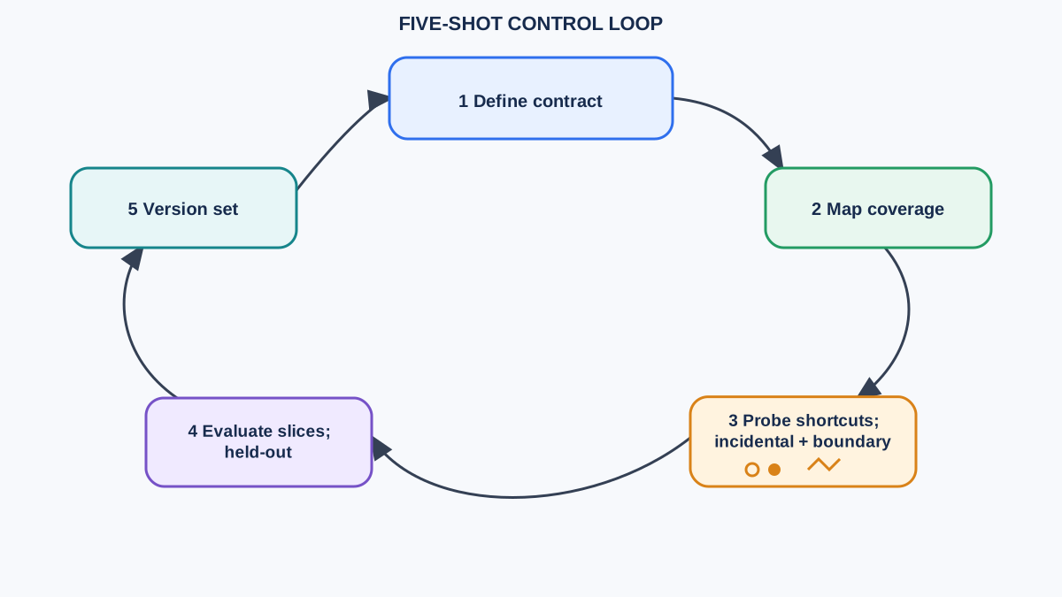
Before selection, ordering, or diversity, name the invariant your set must preserve. A demonstration set is a compressed specification, and a specification has three parts you must be able to state in one sentence each:
- The mapping. The rule that connects an input to its output.
- The decision criterion. The feature that flips the label at the boundary.
- The output contract. The shape, keys, and constraints the response must satisfy.
If you cannot write those three sentences, you cannot predict where the set will fail. Write them down first. Then run the loop:
- State the mapping, criterion, and contract.
- Assign each example a coverage region and a diagnostic job.
- Perturb one incidental feature at a time and observe whether output moves.
- Evaluate on held-out slices, including boundary regions.
- Version the set as an artifact with its own identifier.
Everything below is a stage in that loop. The rest of this article walks each stage and shows what to measure at the end of it.
Knowledge check
Check your understanding
Answer this question before you continue.
What a Demonstration Actually Teaches
Every example carries at least three separable signals, and the model has no built-in way to know which one you care about:
- Surface format. The shape of the output: JSON keys, casing, punctuation, section order, length conventions.
- The input-to-output mapping. The actual rule that connects an input to its label or answer.
- Incidental features. Everything else that happens to correlate with the target across your examples — answer length, tone, label position, a recurring keyword, the order in which classes appear.
You intend to teach the mapping. The model fits the cheapest consistent pattern across all three. If every positive example is longer than every negative one, length becomes a feature. If the label "urgent" always appears last in your list, position becomes a feature. The model is not being lazy; it is being efficient. It finds the lowest-cost rule that explains your demonstrations, and sometimes that rule is not the one you wrote down.
This is why a set can nail the format and still teach the wrong rule. Format compliance is easy to verify and easy to mistake for correctness. A model that returns perfectly structured JSON with the wrong label has learned your schema and missed your task.
A demonstration set is a compressed specification. If the specification is ambiguous, the model resolves the ambiguity — not you.
Selection: Choosing Examples That Carry the Rule
Most weak example sets are assembled by grabbing the first N correct outputs from a dataset. That optimizes for availability, not coverage. Selection should start from the decision boundary: the input regions where the correct output changes.
Enumerate those regions first. For a support-ticket classifier, the regions might be "billing dispute," "feature request," "outage report," and "ambiguous complaint." Then pick one example that clearly marks each region. An example earns its place only if you can name the specific region it disambiguates. If you cannot, it is decoration.
Two selection hazards dominate.
Label skew teaches priors, not rules. If 80% of your examples are one class, the model may learn "usually label X" instead of the criterion that separates X from Y. Balance is not about matching the real-world distribution; it is about giving each boundary enough evidence to be learnable.
Similarity retrieval can collapse into near-duplicates. Dynamic few-shot example selection — retrieving the nearest training examples to the current query via embeddings or KNN — is a reasonable strategy when your input distribution is wide. Its failure mode is subtle: the nearest neighbors to a query are often near-duplicates of each other. You spend context budget on three examples that say the same thing and cover one region. Retrieval optimizes for similarity to the query, not for coverage of the boundary. Those are different objectives, and the second one is usually what you need.
Cost is real. Every example consumes context and attention. More examples are not monotonically better; past a point, additional examples dilute the signal and amplify whatever pattern they share. I treat each example as a line item: if it does not change behavior on some input region, it is paying rent without doing work.
Knowledge check
Check your understanding
Answer this question before you continue.
Ordering: A Hypothesis, Not a Law
The same examples in a different order can produce different behavior. That much is observable. What causes the shift is less settled, and the honest framing is that you are testing a hypothesis, not applying a rule.
Three candidate explanations compete:
- Recency weighting. Later positions weigh more heavily on the immediate continuation, so the example closest to the query dominates format and answer shape.
- Pattern induction. The order itself becomes a feature. Alternate the labels and the model may learn alternation. Sort by length and length becomes a feature.
- Template interaction. The chat template, system prompt, and decoding settings interact with position in ways that vary by model and runtime.
Any of these can be true for a given model, template, and task. None of them is a universal law you can design around without measuring. The practical move is to treat ordering as a variable you control and test, not a property you assume.
Two controls are worth building into your workflow:
- Randomize order across evaluation runs. If accuracy swings meaningfully when you shuffle, your set is order-sensitive and you have been reporting a lucky arrangement as a result.
- Place deliberately when you have a reason. If one example is the most representative of the task, putting it last is a legitimate choice — as long as you know you made it and can defend it.
The reproducibility rule is simple: report ordering as part of the prompt specification. An unreported order is an unreproducible result. When a teammate reruns your prompt and gets different output, the first question is whether the examples were in the same sequence.
Diversity: Covering the Space Without Teaching Noise
Diversity is easy to measure badly. Surface variety — different topics, lengths, and vocabulary — feels diverse and often is not. The diversity that matters is coverage of the decision boundary. Two examples from different domains that exercise the same rule are redundant; two examples from the same domain that exercise different rules are not.
Redundancy has a documented cost. Research on synthetic example generation found that multi-example prompts tend to produce outputs that mirror one of the provided examples, and that larger example sets can suffer from repetition of a single form, making the effective signal less diverse than the set appears. The model latches onto one example and echoes it. Adding more examples of the same shape does not fix this; it deepens it.
The opposite failure is just as damaging. Contradictory examples — same input shape, different labels, no stated distinguishing rule — teach the model that the mapping is arbitrary. When the boundary is genuinely ambiguous, the fix is not more examples. It is an explicit criterion in the instructions that tells the model which feature decides the case.
A coverage table makes both failures visible. Rows are input regions; columns are your examples. Mark which example covers which region, then look for empty cells (under-coverage) and over-filled cells (redundancy).
| Input region | Ex. 1 | Ex. 2 | Ex. 3 | Ex. 4 |
|---|---|---|---|---|
| Billing dispute | ✓ | ✓ | ||
| Feature request | ✓ | |||
| Outage report | ✓ | |||
| Ambiguous complaint |
The empty row is your next example. The double-checked row is a candidate for deletion.
Boundary Cases: The Examples That Do the Real Work
Boundary examples are where the mapping gets pinned down. Define the boundary as the set of inputs where a naive rule and your intended rule disagree. Those are the inputs that separate a model that learned your task from one that learned a shortcut.
Near-misses do the heaviest lifting. A near-miss is an input that looks like class A but is class B — the support ticket that reads like a feature request but is actually a bug report, the review that sounds negative but recommends the product. Near-misses force the model to use the actual criterion instead of a surface cue. If adding a near-miss changes behavior on your eval set, your earlier examples were teaching a shortcut, and you just found it.
A boundary pair is stronger than a single boundary example. Construct two inputs that differ in exactly one feature — the criterion-relevant one — and label them differently. That pair teaches the model which feature flips the label. A single boundary example only shows that a region exists; a pair shows what decides it.
Boundary examples are diagnostic instruments. Each one you add is a test of whether the rest of your set was honest.
One caution: boundary examples are also the easiest place to introduce label ambiguity. A near-miss that you cannot confidently label is not a boundary example; it is a coin flip that will teach the model to guess. Verify each one is genuinely unambiguous before it goes in.
Abstention and Refusal Are a Separate Problem
If your task has an abstention or rejection behavior — a "cannot answer" or "out of scope" output that is part of the application's contract — you can demonstrate it with a contrast pair: one example that should be answered, one that should be rejected, differing only in the feature that triggers abstention. That teaches the task-level criterion.
This is not the same as safety policy. Model-level refusal, content filtering, and access control are governed by higher-level instructions, model policy, and application logic — not by demonstrations. Adding a refusal example does not make a model safe, and it can teach over-refusal if the contrast is weak. If you add one, add an over-refusal eval slice alongside it and measure both directions.
Knowledge check
Check your understanding
Answer this question before you continue.
Avoiding Accidental Correlations
The audit question is one sentence: what feature is perfectly correlated with the label across my examples but is not part of the task?
Common culprits:
- Answer length (positives longer than negatives)
- Sentiment or tone that tracks the label without being the criterion
- Formatting differences between classes
- Position in the list
- A specific keyword that appears in one class
- Label frequency
Two tests find them.
The counterfactual test. Take a correct example, change only the incidental feature, and check whether the model's output changes. Lengthen a positive example. Strip the keyword. Move it to a different position. If the output flips, the incidental feature was load-bearing.
The ablation test. Remove one example at a time and measure the delta on your eval set. Examples that change nothing are candidates for deletion. Examples whose removal causes a large drop are carrying the rule — keep them and understand why. Ablation shows dependence, not causal necessity; an example can matter because it is redundant with another, and removing both may hurt more than removing either alone.
Not every correlation is spurious. Some features genuinely track the label because they are part of the task. The distinction is whether the feature would still predict the label on inputs you have not seen. If it would, it is signal. If it only holds inside your example set, it is a trap. When the boundary is genuinely ambiguous, state the criterion explicitly in the instructions rather than hoping the examples imply it.
Knowledge check
Check your understanding
Answer this question before you continue.
Evaluating the Example Set, Not Just the Prompt
You cannot tell whether a demonstration set is working by looking at it. You measure it.
Build a small labeled eval set that deliberately includes boundary cases, not just typical inputs. Then run a controlled comparison. Hold the model, instructions, decoding settings, and prompt template fixed. Change one variable per run. If sampling is enabled, repeat each configuration enough times to see the spread, not just the mean.
| Configuration | Variable changed | Typical slice | Boundary slice | Format compliance |
|---|---|---|---|---|
| Zero-shot | — | |||
| One-shot | example count | |||
| Curated set | example content | |||
| Shuffled order | ordering only | |||
| Ablated set | one example removed |
The deltas tell you what the examples are actually contributing. If your curated set barely beats zero-shot, the examples are not carrying the rule — the instructions are, and you are paying context for nothing. If the shuffled variant diverges sharply, your result depends on ordering. If the ablated set holds steady, the removed example was not doing work.
Track per-region accuracy, not just aggregate. A set can score well overall while failing an entire boundary region, because the typical inputs outnumber the hard ones. Aggregate accuracy hides exactly the failures you built the set to prevent.
Version the example set as an artifact with its own identifier. When behavior changes after a model update, you need to attribute the change to the set, the instructions, or the model — and you cannot do that if the set is a pile of pasted outputs with no history. Hold instructions fixed while varying examples, then hold examples fixed while varying instructions. Otherwise the result is unattributable.
When Few-Shot Examples Are the Wrong Tool
Examples are not always the answer, and adding them can be the wrong move. Each of these is a measurable decision test, not a vibe:
- No correctness or format delta. If your curated set does not beat zero-shot on the eval slices you care about, the examples are not carrying signal. Remove them and reclaim the context.
- High per-call cost with a stable rule. If the rule is fixed and you are paying for it on every call, fine-tuning may be a better home for the signal than a growing prompt.
- Unstable input distribution. A static example set decays. The real problem becomes dynamic selection or retrieval, which is a different design space.
- Capability failure despite representative examples. If the model cannot do the task at all, more examples will not teach it. You are describing a capability gap, not a specification gap.
The hand-off is worth naming. Once examples must be selected at runtime per query, you have moved from prompt engineering into context assembly and orchestration. A production selector looks roughly like this:
candidate pool (offline artifact)
  -> query-conditioned retrieval (per request)
  -> redundancy / boundary filter (per request)
  -> ordering policy (per request)
  -> rendered demonstrations (per request)
  -> slice-based evaluation (offline, on held-out data)
The candidate pool and the evaluation harness are offline artifacts you own and version. Retrieval, filtering, and ordering run per request and must be cheap. Keeping that boundary explicit is what stops a prompt-engineering problem from quietly becoming an unmonitored retrieval system.
What to Do Next
Pick one example set you currently rely on and audit it this week.
Write the three sentences: the mapping, the decision criterion, the output contract. Then run the counterfactual test on each example: change one incidental feature and see whether the output moves. Run the ablation test: remove one example at a time and measure the delta on a held-out slice that includes boundary cases. Delete the examples that change nothing. Add one boundary pair that differs only in the criterion-relevant feature. Re-measure per-region accuracy, not just the aggregate.
Treat the result as a versioned artifact you own and can defend — not a pile of pasted outputs. The set is the specification. Make it say what you mean, then prove it does.
Knowledge check
Final check
Finish the article by checking the ideas you just learned.
References
Research updated Sep 11, 2026


